Preparation
In order to query SNMP data I had to install some Debian packages:
/install-packages.sh
sudo apt-get install \
  snmp \
  snmp-mibs-downloader
snmp package provides the required command line tools, especially snmpget and snmpwalk.
snmp-mibs-downloader provides Management Information Base files in the directory /usr/share/snmp/mibs SNMP data structures.SNMP structures the management information in a numerical, hierarchical format that is very hard to reason about:
/snmpwalk.sh
snmpwalk -v2c -c public 10.0.0.3
iso.3.6.1.2.1.1.1.0 = STRING: "Linux bay5 3.2.0-59-generic #90-Ubuntu SMP Tue Jan 7 22:43:51 UTC 2014 x86_64"
iso.3.6.1.2.1.1.2.0 = OID: iso.3.6.1.4.1.8072.3.2.10
iso.3.6.1.2.1.1.3.0 = Timeticks: (145234) 0:24:12.34
iso.3.6.1.2.1.1.4.0 = STRING: "Root <root@localhost>"
iso.3.6.1.2.1.1.5.0 = STRING: "bay5"
iso.3.6.1.2.1.1.6.0 = STRING: "Server Room"
iso.3.6.1.2.1.1.8.0 = Timeticks: (0) 0:00:00.00
iso.3.6.1.2.1.1.9.1.2.1 = OID: iso.3.6.1.6.3.10.3.1.1
iso.3.6.1.2.1.1.9.1.2.2 = OID: iso.3.6.1.6.3.11.3.1.1
iso.3.6.1.2.1.1.9.1.2.3 = OID: iso.3.6.1.6.3.15.2.1.1
iso.3.6.1.2.1.1.9.1.2.4 = OID: iso.3.6.1.6.3.1
iso.3.6.1.2.1.1.9.1.2.5 = OID: iso.3.6.1.2.1.49
iso.3.6.1.2.1.1.9.1.2.6 = OID: iso.3.6.1.2.1.4
iso.3.6.1.2.1.1.9.1.2.7 = OID: iso.3.6.1.2.1.50
iso.3.6.1.2.1.1.9.1.2.8 = OID: iso.3.6.1.6.3.16.2.2.1
iso.3.6.1.2.1.1.9.1.3.1 = STRING: "The SNMP Management Architecture MIB."
iso.3.6.1.2.1.1.9.1.3.2 = STRING: "The MIB for Message Processing and Dispatching."
iso.3.6.1.2.1.1.9.1.3.3 = STRING: "The management information definitions for the SNMP User-based Security Model."
iso.3.6.1.2.1.1.9.1.3.4 = STRING: "The MIB module for SNMPv2 entities"
iso.3.6.1.2.1.1.9.1.3.5 = STRING: "The MIB module for managing TCP implementations"
iso.3.6.1.2.1.1.9.1.3.6 = STRING: "The MIB module for managing IP and ICMP implementations"
iso.3.6.1.2.1.1.9.1.3.7 = STRING: "The MIB module for managing UDP implementations"
iso.3.6.1.2.1.1.9.1.3.8 = STRING: "View-based Access Control Model for SNMP."
# ~2300 more entries
MIBS environment variable:
/capture-snmp.sh
export MIBS=ALL
/snmpwalk-mibs.sh
$ snmpwalk -v2c -c public 10.0.0.3
SNMPv2-MIB::sysDescr.0 = STRING: Linux bay5 3.2.0-59-generic #90-Ubuntu SMP Tue Jan 7 22:43:51 UTC 2014 x86_64
SNMPv2-MIB::sysObjectID.0 = OID: NET-SNMP-TC::linux
DISMAN-EVENT-MIB::sysUpTimeInstance = Timeticks: (201014) 0:33:30.14
SNMPv2-MIB::sysContact.0 = STRING: Root <root@localhost>
SNMPv2-MIB::sysName.0 = STRING: bay5
SNMPv2-MIB::sysLocation.0 = STRING: Server Room
SNMPv2-MIB::sysORLastChange.0 = Timeticks: (0) 0:00:00.00
SNMPv2-MIB::sysORID.1 = OID: SNMP-FRAMEWORK-MIB::snmpFrameworkMIBCompliance
SNMPv2-MIB::sysORID.2 = OID: SNMP-MPD-MIB::snmpMPDCompliance
SNMPv2-MIB::sysORID.3 = OID: SNMP-USER-BASED-SM-MIB::usmMIBCompliance
SNMPv2-MIB::sysORID.4 = OID: SNMPv2-MIB::snmpMIB
SNMPv2-MIB::sysORID.5 = OID: TCP-MIB::tcpMIB
SNMPv2-MIB::sysORID.6 = OID: RFC1213-MIB::ip
SNMPv2-MIB::sysORID.7 = OID: UDP-MIB::udpMIB
SNMPv2-MIB::sysORID.8 = OID: SNMP-VIEW-BASED-ACM-MIB::vacmBasicGroup
SNMPv2-MIB::sysORDescr.1 = STRING: The SNMP Management Architecture MIB.
SNMPv2-MIB::sysORDescr.2 = STRING: The MIB for Message Processing and Dispatching.
SNMPv2-MIB::sysORDescr.3 = STRING: The management information definitions for the SNMP User-based Security Model.
SNMPv2-MIB::sysORDescr.4 = STRING: The MIB module for SNMPv2 entities
SNMPv2-MIB::sysORDescr.5 = STRING: The MIB module for managing TCP implementations
SNMPv2-MIB::sysORDescr.6 = STRING: The MIB module for managing IP and ICMP implementations
SNMPv2-MIB::sysORDescr.7 = STRING: The MIB module for managing UDP implementations
SNMPv2-MIB::sysORDescr.8 = STRING: View-based Access Control Model for SNMP.
# ~2300 more entries
systemStats or memory:
/capture-snmp.sh
snmpwalk -v2c -c public 10.0.0.3 systemStats > 10.0.0.3.systemStats.snmpwalk
snmpwalk -v2c -c public 10.0.0.3 memory      > 10.0.0.3.memory.snmpwalk
/10.0.0.3.systemStats.snmpwalk
UCD-SNMP-MIB::ssIndex.0 = INTEGER: 1
UCD-SNMP-MIB::ssErrorName.0 = STRING: systemStats
UCD-SNMP-MIB::ssSwapIn.0 = INTEGER: 0 kB
UCD-SNMP-MIB::ssSwapOut.0 = INTEGER: 0 kB
UCD-SNMP-MIB::ssIOSent.0 = INTEGER: 6 blocks/s
UCD-SNMP-MIB::ssIOReceive.0 = INTEGER: 0 blocks/s
UCD-SNMP-MIB::ssSysInterrupts.0 = INTEGER: 62 interrupts/s
UCD-SNMP-MIB::ssSysContext.0 = INTEGER: 124 switches/s
UCD-SNMP-MIB::ssCpuUser.0 = INTEGER: 1
UCD-SNMP-MIB::ssCpuSystem.0 = INTEGER: 0
UCD-SNMP-MIB::ssCpuIdle.0 = INTEGER: 97
UCD-SNMP-MIB::ssCpuRawUser.0 = Counter32: 3112
UCD-SNMP-MIB::ssCpuRawNice.0 = Counter32: 0
UCD-SNMP-MIB::ssCpuRawSystem.0 = Counter32: 366
UCD-SNMP-MIB::ssCpuRawIdle.0 = Counter32: 16735
UCD-SNMP-MIB::ssCpuRawWait.0 = Counter32: 96
UCD-SNMP-MIB::ssCpuRawKernel.0 = Counter32: 0
UCD-SNMP-MIB::ssCpuRawInterrupt.0 = Counter32: 33
UCD-SNMP-MIB::ssIORawSent.0 = Counter32: 5482
UCD-SNMP-MIB::ssIORawReceived.0 = Counter32: 203276
UCD-SNMP-MIB::ssRawInterrupts.0 = Counter32: 31382
UCD-SNMP-MIB::ssRawContexts.0 = Counter32: 68221
UCD-SNMP-MIB::ssCpuRawSoftIRQ.0 = Counter32: 13
UCD-SNMP-MIB::ssRawSwapIn.0 = Counter32: 0
UCD-SNMP-MIB::ssRawSwapOut.0 = Counter32: 0
/10.0.0.3.memory.snmpwalk
UCD-SNMP-MIB::memIndex.0 = INTEGER: 0
UCD-SNMP-MIB::memErrorName.0 = STRING: swap
UCD-SNMP-MIB::memTotalSwap.0 = INTEGER: 466936 kB
UCD-SNMP-MIB::memAvailSwap.0 = INTEGER: 466936 kB
UCD-SNMP-MIB::memTotalReal.0 = INTEGER: 1026948 kB
UCD-SNMP-MIB::memAvailReal.0 = INTEGER: 632672 kB
UCD-SNMP-MIB::memTotalFree.0 = INTEGER: 1099608 kB
UCD-SNMP-MIB::memMinimumSwap.0 = INTEGER: 16000 kB
UCD-SNMP-MIB::memBuffer.0 = INTEGER: 4116 kB
UCD-SNMP-MIB::memCached.0 = INTEGER: 97152 kB
UCD-SNMP-MIB::memSwapError.0 = INTEGER: noError(0)
UCD-SNMP-MIB::memSwapErrorMsg.0 = STRING:
Capturing Data Regularly
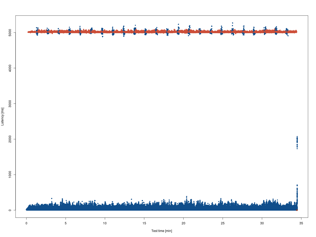
As a first step, I was fine with just capturing CPU and memory statistics. Selectively querying this information was quite valueable, because a fullsnmpwalk turned out to be too expensive and influenced the test results.
I wrote a small script to record systemStats and memory every 60 seconds:
/capture-snmp-regularly.sh
host=$1
interval=${2:-60}

export MIBS=ALL
while true; do
  timestamp=$(date +%s%N | cut -b1-13)
  record_dir="$host/$timestamp"
  echo "Recording SNMP indicators to $record_dir/"
  mkdir --parents "$record_dir"
  snmpwalk -t 1 -v2c -c public $host systemStats > $record_dir/$host.systemStats.snmpwalk
  snmpwalk -t 1 -v2c -c public $host memory      > $record_dir/$host.memory.snmpwalk
  sleep $interval
done
Cleaning Up and Collecting the Captured Data
To prepare the data for analysis with R, I stripped out some uninteresting tokens:
/cleanup-snmp-data.sh
#!/bin/bash
cat - | \
  sed "s/UCD-SNMP-MIB:://" | \
  sed "s/INTEGER: //" | \
  sed "s/STRING: //" | \
  sed "s/Counter32: //" | \
  sed "s/\.0//" | \
  sed "s/ = /,/g"
snmpwalk data, clean it up and prepending the host name and timestamp.
/collect-snmp-data.sh
#!/bin/bash
for recording in $( ls --directory */*/ ); do
  host=$( echo "$recording" | sed 's/\([0-9]\+\.[0-9]\+\.[0-9]\+\.[0-9]\+\)\/\([0-9]\+\)\//\1/' )
  timestamp=$( echo "$recording" | sed 's/\([0-9]\+\.[0-9]\+\.[0-9]\+\.[0-9]\+\)\/\([0-9]\+\)\//\2/' )
  cat $host/$timestamp/*.snmpwalk | ./cleanup-snmp-data.sh | sed "s/^/$host,$timestamp,/"
done
./collect-snmp-data > snmp.csv produces a neat CSV file, ready for R.Plotting the Data
Finally, I plotted the data with R.
/snmp.R
snmps<-read.table("snmp.csv",
                  header=FALSE,
                  col.names=c('host','timestamp','valueType','value'),
                  colClasses=c('factor','numeric','factor','character'),
                  sep=","
)
ssCpuUser<-snmps[ snmps$valueType == 'ssCpuUser', ]
plot((ssCpuUser$timestamp-min(ssCpuUser$timestamp))/1000/60,
     ssCpuUser$value,
     type='o',
     main=expression(bold(paste(ssCpuUser, ", ", 1-textstyle(frac(memAvailReal, memTotalReal))))),
     xlab="Test time [min]",
     ylab="Utilization [%]",
     ylim=c(0,100),
     col="purple",
     pch=18
)

timestamps<-snmps[ snmps$valueType == 'memTotalReal', ]$timestamp
memTotalReal<-as.numeric(sub("([0-9]+) kB", "\\1", snmps[ snmps$valueType == 'memTotalReal', ]$value))
memAvailReal<-as.numeric(sub("([0-9]+) kB", "\\1", snmps[ snmps$valueType == 'memAvailReal', ]$value))
reservedMem<-1-memAvailReal/memTotalReal

lines((timestamps-min(timestamps))/1000/60,
      reservedMem*100,
      type='o',
      ylim=c(0,100),
      col="orange",
      pch=18
)
legend(0, 20,
       c("ssCpuUser", expression(1-textstyle(frac(memAvailReal, memTotalReal)))),
       col=c("purple", "orange"),
       yjust=0.5,
       pch=18
)
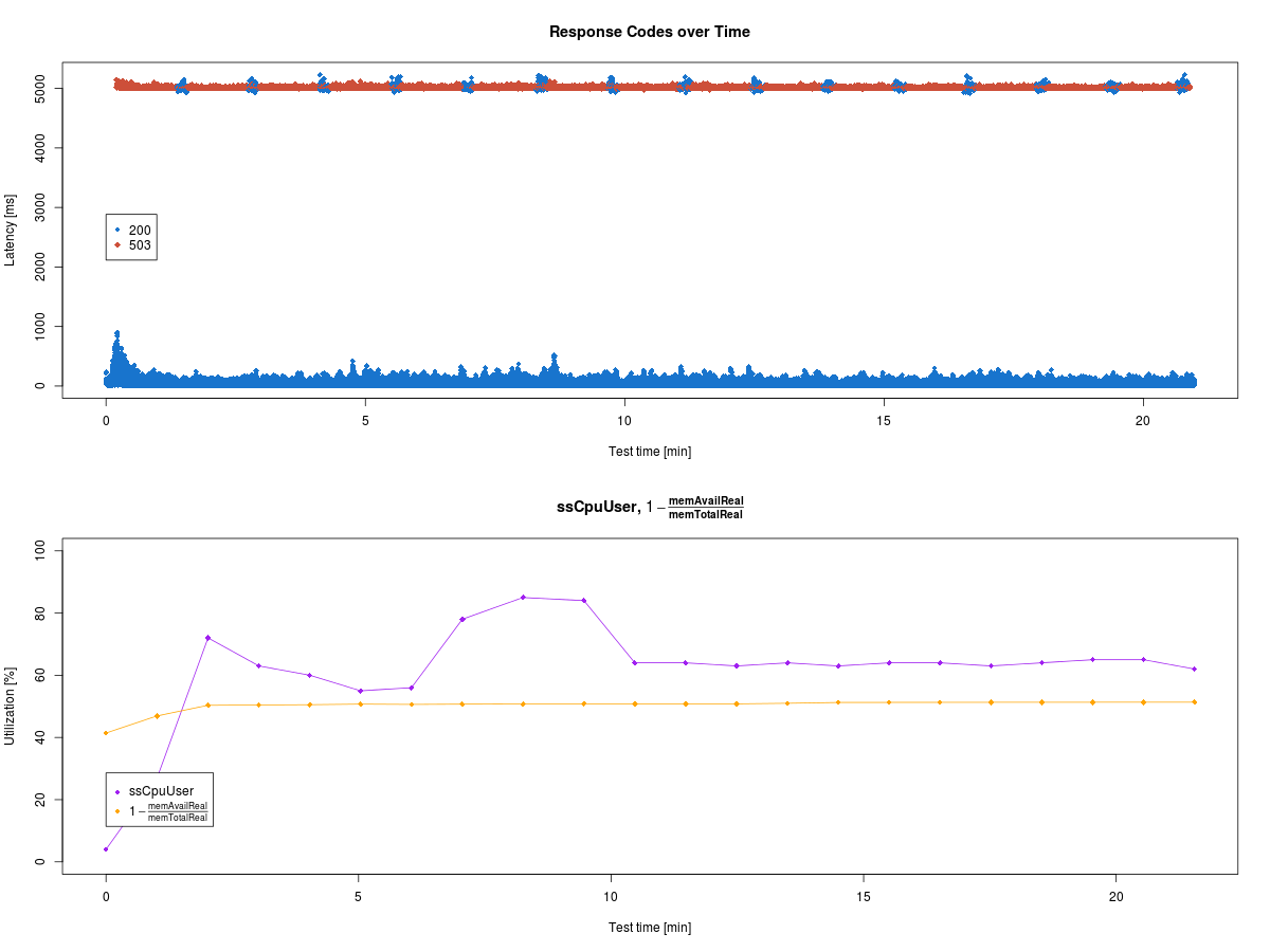
The result does not suggest any relationships between these system parameters and the response times. But that just motivates further investigation. :-) So stay tuned!
As always, the sources are available via GitHub.